With Pivot Tables you can analyze any data in your Equals workbooks without writing formulas. Pivot Tables are particularly powerful in Equals as you can pivot directly off data from your SQL database, data warehouse, Salesforce, or Quickbooks instance.

To create a Pivot Table:

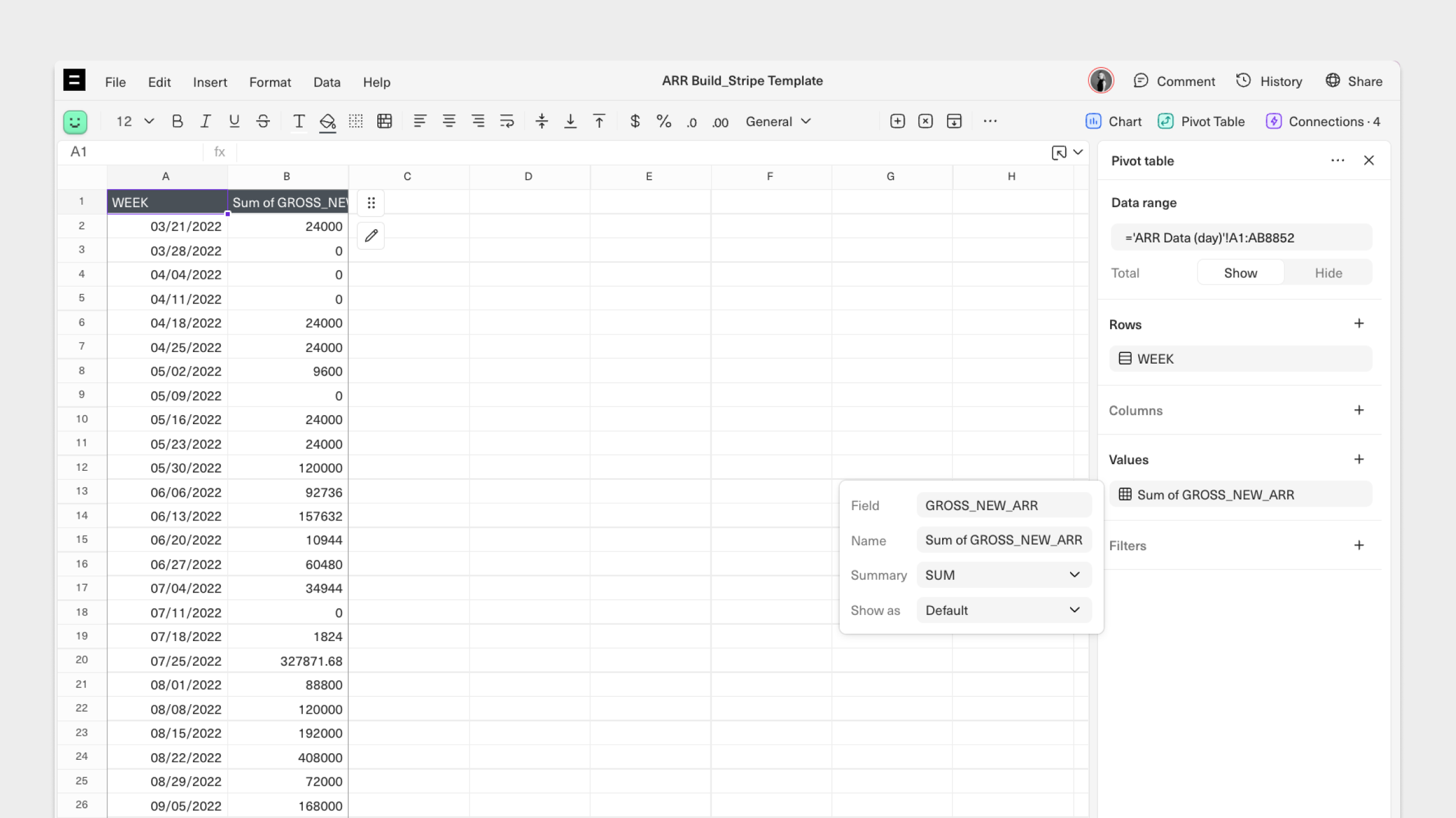
1. Select the data you'd like to analyze, click Insert > Pivot Table. You'll see the Pivot Table configuration sidebar where you can set up your analysis.
2. Select the + button to add fields from your data as rows, columns, or values to be displayed in the pivot.
3. Click on the field to customize the data displayed.

There are multiple ways to summarize your data:

• By adding fields as Rows, you'll generate a unique list of all the values in that field as separate rows.
• By adding fields as Values, you'll be able to choose how to aggregate the data in that field (e.g., sum, count, average, min, max).
• By adding fields as Columns, you can break down pivots by one or more dimensions across separate columns.

Advanced features

Pivot Tables support a number of advanced features: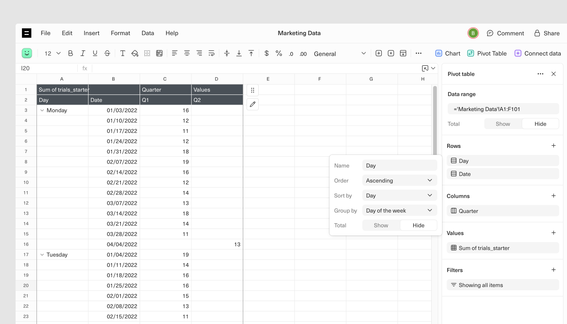

• Sort by can be used to organize your pivot table based on a specific value. Clicking into a field will allow you to use the sort by functionality.
• Totals toggle to show or hide grand totals, can also be handled at the field level. Clicking into a field will allow you adjust this at the field level.
• Calculated Fields can be used to add a field based off the source data. For example, if you had a "Total Spend" field and a "Number of Purchases" field, you could create an "Average Spend" calculated field that divided the first by the second. Use the "Calculated Column" text visible in the drop-down for Rows, Values, or Columns (after clicking on the + button) to create and insert a Calculated Field.
• Summary Functions can be used to summarize your values in different ways. e.g. Sum, Count, Min, Max, etc. To change the Summary Function used, click on a displayed field and choose the function you would like to summarize by.
• Filters can be used to filter an existing analysis. To filter your analysis, click on the + icon next to the Filter section to add a field you’d like to apply a filter over. Note: date filters will not include future dates (ex: if you select “January 2022” on the 4th of January, the 5th of January will not be displayed as the filter will be identical to the selection on the date of pivot creation).