This document captures all the ways to format your workbook, including borders, conditional formatting rules, and custom number formats.

Borders

You can add borders to emphasize a range of cells or single cell in your workbooks.

To get started, click on a cell or a selection of cells. Then, click on the borders icon from the toolbar. This will open a drop down that will allow you to customize how you'd like your borders applied.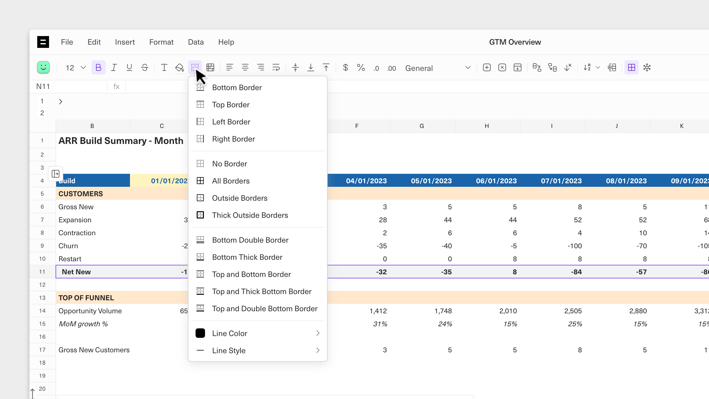

Conditional formatting

Conditional formatting makes it easy to highlight trends or patterns in your data by making cells or values easy to identify. You can use conditional formatting to color-code cells that meet a specific set of criteria.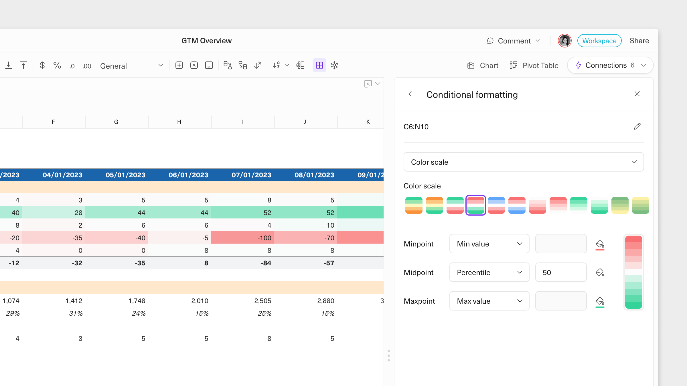

To get started:

Select a cell or a range of cells and click on Format > Conditional Formatting > New Rule from the toolbar.
Set rules for your formatting. You can toggle between the Highlight cell option, which allows you to granularly set the conditions for your formatting, or you can use the Color scale option which will apply shading based on the median value in your data range.

Selecting Manage Rules (Format > Conditional Formatting > Manage Rules) will allow you to view all of the formatting criteria applied in your sheet and make changes.

Custom number formatting

With custom number formatting you can change how your data is displayed. For example, you can set all negative numbers in parentheses or add your currency symbol to spend data.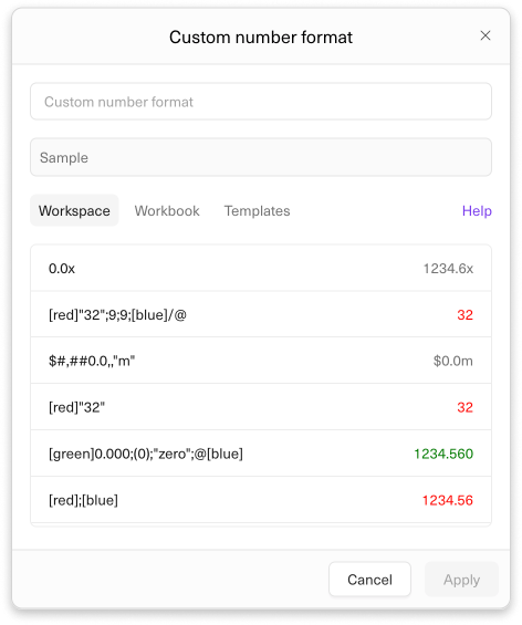

To apply a custom number format to a selection on your sheet:

Click on Format in your workbook's tool bar. This will open a console where you can configure how your data should be presented.
Write a set of rules in the console that will be applied to the data on your sheet. You can specify as many rules as you need. Clicking on "Templates" you'll be able to browse common formattings that you can use as a starting point.

Syntax for setting formats

To use colors in your format, write a color name in brackets (for example, [Blue]) anywhere in the desired part of the format. You must use English color names. The colors that can be used are white, red, blue, green, magenta, yellow, and cyan. You can also use Color#, where the # symbol is a number between 1 and 56 corresponding to the 56 Excel ColorIndex colors.

If you specify a color in the custom format, that color will take precedence over colors selected in the text color picker. The following symbols can be used to format numbers:

Symbol	Result	Example
0	Digit or Zero	`2` formatted with 00 will show `"02"`
#	Digit if needed	`2` formatted with `##` will show `"2"`
?	Digit or Space	`2` formatted with `??` will show `"2"`
.	Decimal point	`1.345` formatted with `#.#` will show `1.3`
,	Thousands separator	`1345` formatted with `#,##0` will show `"1,345"`
%	Percentage	Number is multiplied by 100 before it is shown. `0.3` formatted with `0%` will show `"30%"`
e-, e+	Exponential format	`12200000` formatted with `0.00E+00` will emit `"1.22E+07"`
"text"	Pass-through	Pass through whatever text is inside the quotation marks as-is. `2` formatted with `0 "USD"` will show `"2 USD"`
\	Escape	Pass the the next character through as-is.
$, -, +, /, (, ),	Pass-through	Symbols are printed as-is, without the need to use quotations or escape characters
@.	Text value	When value is non-numeric, show it as is. `two` formatted with `"one"@"three"` will emit `"onetwothree"`

Symbol	Result	Example
yy	Two digit year	23
yyyy	Four digit year	2023
m	Month	1
mm	Two digit month	01
mmm	Month name abbreviation	Jan
mmmm	Full month name	January
mmmmm	Single letter month abbreviation	J
d	Days	1-31
dd	Days	01-31
ddd	Weekday abbreviation	Wed
dddd	Full weekday name	Wednesday
h	Hours	0–23 or 1–12
hh	Hours	00–23 or 01–12
m	Minutes	0–59
mm	Minutes	00–59
s	Seconds	0–59
ss	Seconds	00–59
AM/PM	12h clock	Sets clock to 12h and emits AM or PM
A/P	12h clock	Sets clock to 12h and emits A or P
[h]	Hours	Elapsed time in hours
[m]	Minutes	Elapsed time in minutes
[s]	Seconds	Elapsed time in seconds